
Plotting Method |
Four curve types are available
Polyline
Hyperbolic and its corrected curve
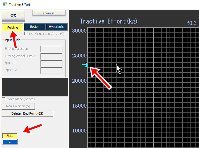
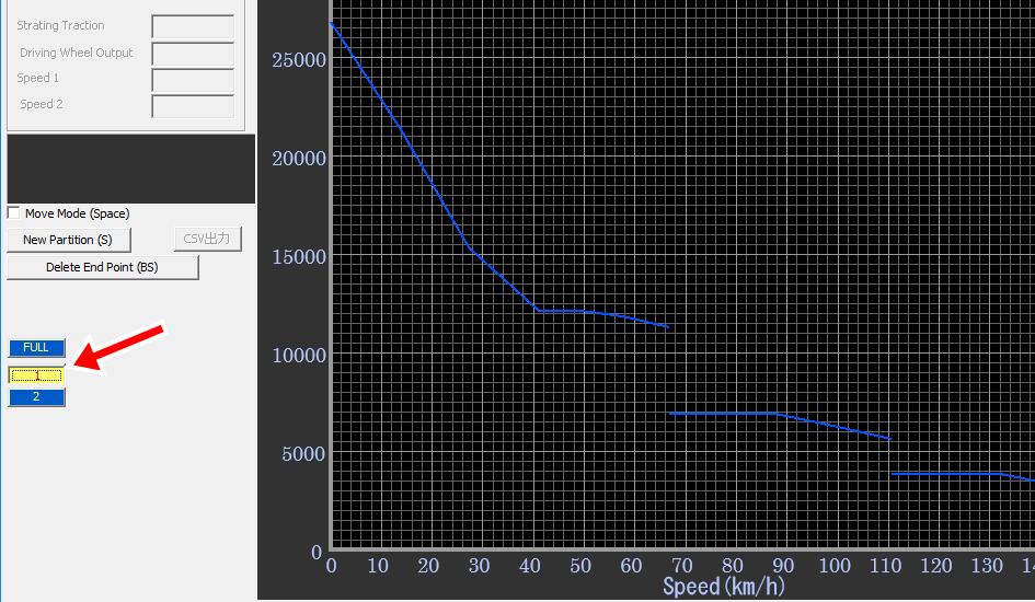
Click "Polyline" button and "FULL" button.
Move the mouse pointer into the graph area and then the sky blue arrow is
displayed at the vertical axis.
This specifies the starting traction.
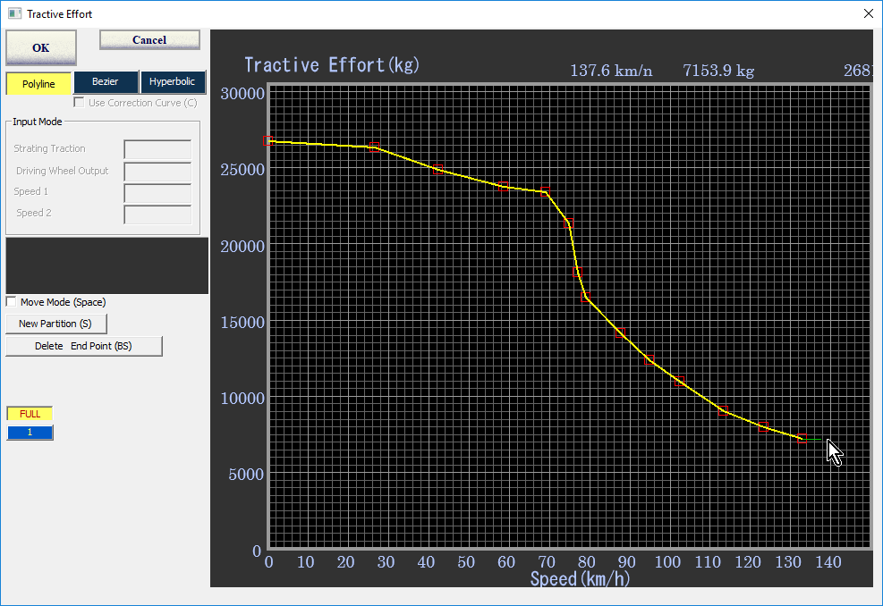
Click speed-traction data one after another.
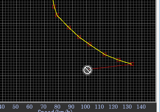
You must plot data from left to right. If not, the mouse pointer turns into "Forbidden".
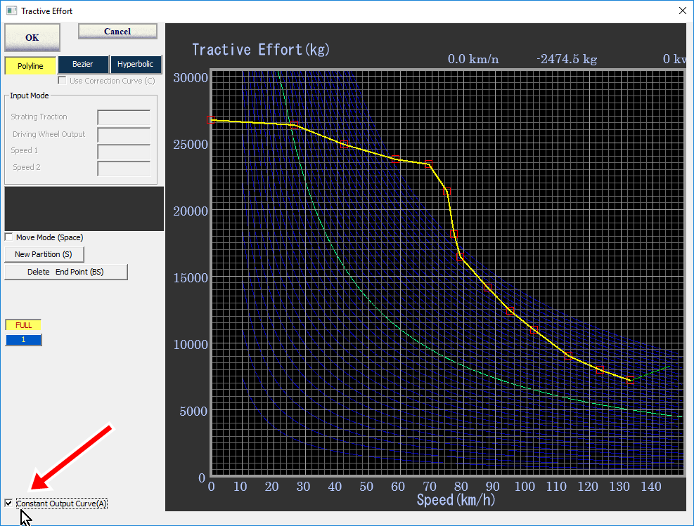
When "Constant Output Curve(A)" is checked, the constant output
curve is displayed on the graph.
This can be switched by "A" key
.
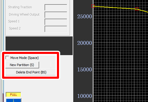
Click "Delete End Point(BS)" button, then the terminal point data is deleted one by one. "Delete" key and "Back Space" key have the same function.
When "Move Mode(Space) is checked, the mode of the input method turns
into the move mode and the mouse pointer changes to "Move" when the
pointer is near at a plotted point..
In this condition, the plotted point can be moved by dragging.
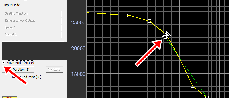
This mode can be switched by pressing the space key.
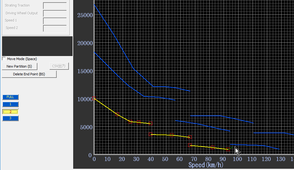
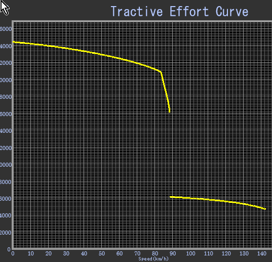
"New partition(S)" is used to generate discontinuous lines for gear type transmissions whose output torque is discontinuous.
Click this button or press "S" key.
Then new starting section is specified by the sky blue arrow.
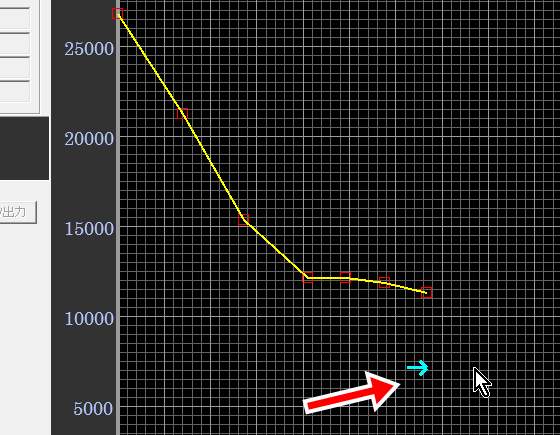
Then plot the data of the new section.
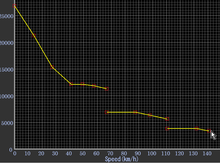
Specify the curve type and the notch number. The notch number 0 is automatically defined as "Full" notch position.
Click "1" button and then new "2" button appears below "1" button and the plotted curves turns into blue.
Plot the data as described above.
You can plot up to 19 notches.
Click "Bezier" button and then plot three points.
Then green curve appears on the graph area.
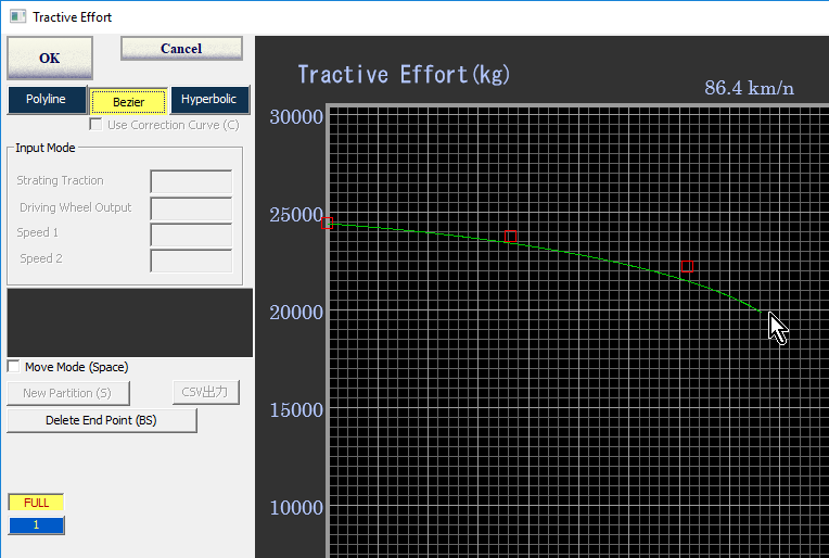
Bezier curve is controlled by 4 points so that you can change the shape by moving mouse pointer.
Click and determine the 4th point and then new curve section starts.
Methods to change data and generate discontinuous curves are same as the polyline described above.
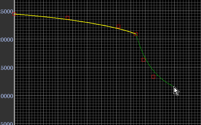
As there is no plotting limitation in Bezier curve mode, you can even plot the curve like this.
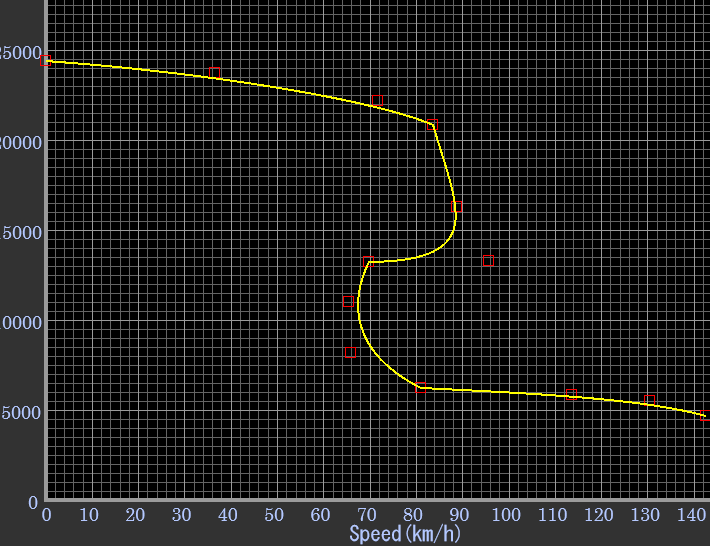
In such a case the turned back region is ignored and the tractive effort is generated like this.
Using this function, you can plot the theoretical performance curve of
an electric motor easily.
The theoretical performance curve of an electric motor consists of three parts.
The first is the constant torque region (red section), and the second is the
constant output region (green section) and the third is the high speed region
(yellow section).
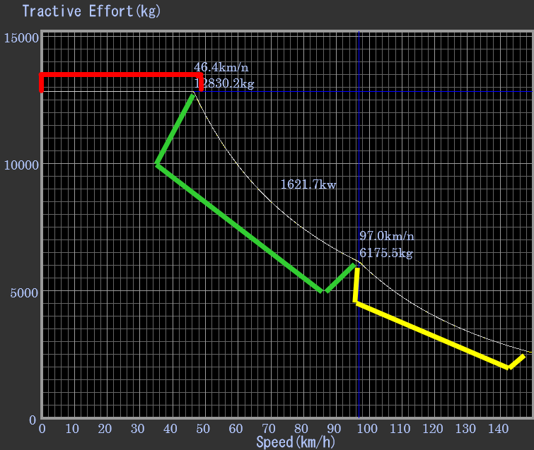
The shape of the curve is determined by the starting traction, the output of motor and the starting speed of the high speed region.
By changing these data at the edit boxes, you can get the performance curve very easily.
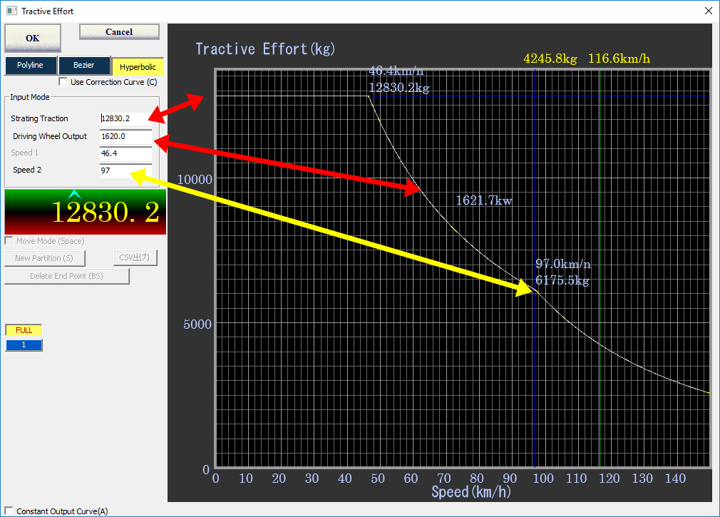
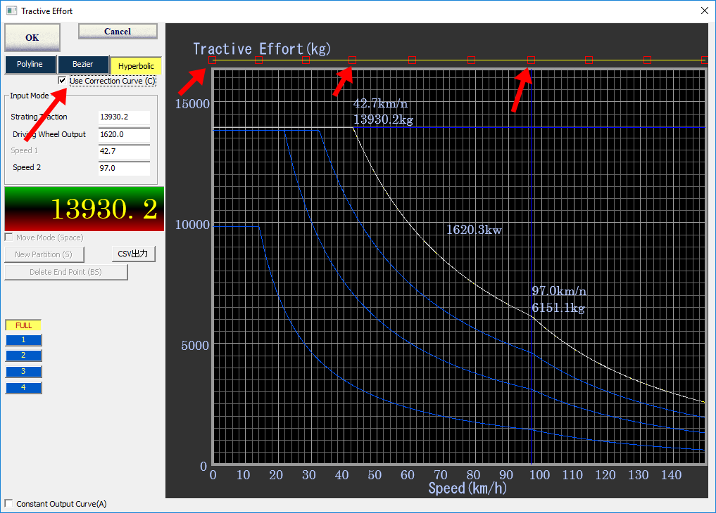
How to edit values with your mouse
In the real world, the performance curve is deviated from the theoretical
curve due to the electrical or magnetic loss and the setting of the electric
controller.
Super Notch Man has the function to adjust this deviation using Bezier curves.
Click "Use Correction Curve(C)" or press "C" key and then the Bezier curve consists of three nodes is displayed at the top of the graph area.
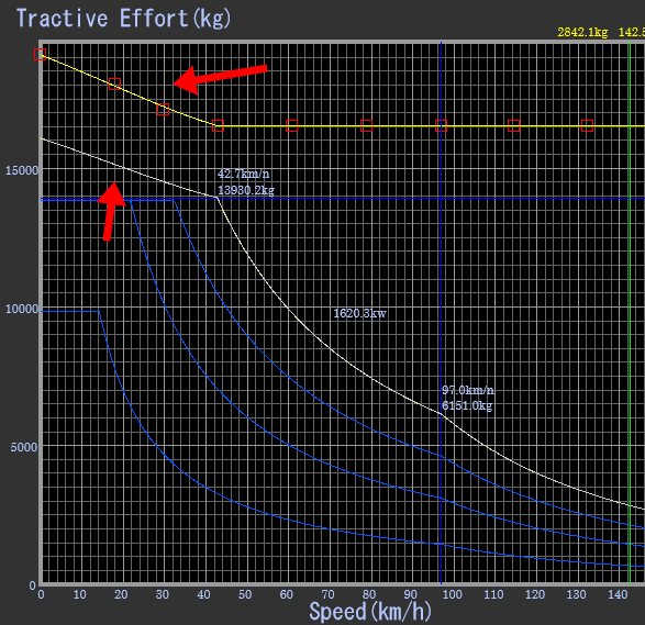
When the mouse pointer points at the control point of Bezier curve, the red
frame turns its color to green and in this state, you can drag the control point
and change the shape of Bezier curve.
When Bezier curve changes, the shape of the performance curve changes.
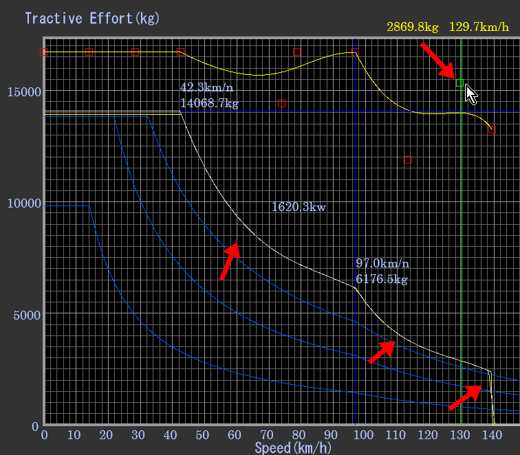
When the traction control is applied and the curve shape of the constant torque region is deformed, you can use this function like this.
©2021 JETconnect Co,. LTD All rights reserved.